Hyperparameter tuning with R's tfruns package

Motivation

Hyperparameter tuning, the process of choosing parameter values within a model, is an essential step for training AI/ML models. For neural networks, choice of hyperparameter values such as dropout rates for each layer, type of optimizer, and numer of nodes can make a huge impact performance. Unfortunately, there are ‘rules of thumb’ for these at best, so it is often better to let the data inform what values to choose.

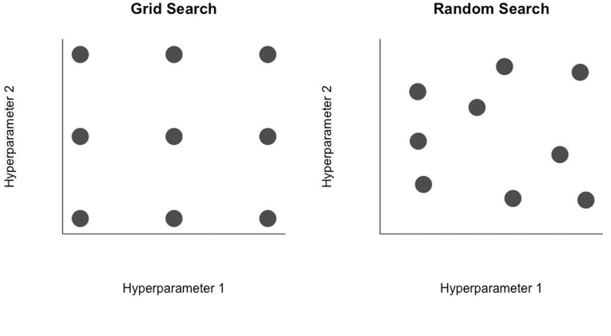
In the case of two hyperparameters, one could systematically search over a grid of candidate values (top left), selecting the pair of values that lead to the best performing model. Or to remove a layer of subjectivity, a random search (top right) may be better. Regardless, even with two hyperparemeters it is easy to see how the number of potential combinations is very large, a challenge for neural networks that are expensive to retrain. In reality, even simple networks can have a few dozen hyperparameters, and some of the more complex networks have tens of thousands to millions of hyperparameters. The curse of dimensionality makes searching across this variable space for strong candidates very difficult.

To tackle the challenge of optimizing hyperparemeter search, many more advanced algorithms than grid or random search have been proposed and implemented, such as a Bayesian optimization, which uses past evaluations of hyperparameter values to update the prior and inform prospective hyperparameter choices. Google even has an AutoML suite service for hyperparameter tuning.

Here I will explore how to manage all of the runs generated from a hyperparameter search using R’s tfruns package. It can be used for manual search, grid search, and random search quite flexibly.

TensorFlow’s tfruns package

I came across the tfruns package recently and used it to train the RiverHeatNet river temperature model and found it incredibly handy. The package is created by the TensorFlow community. The package is designed to help:

• Systematically store hyperparameter values, performance metrics, and source code of each run
• Identify the best performing model across a set of training runs
• Visualize and summarize training run performance

If you have a network coded in Keras already, there are only a few tweaks necessary to make it compatible.

Step 0: Select hyperparameters

In a perfect world you could search across all of the hyperparameters of your model at a great deal of granularity. However, most of us do not have free access to supercomputer resources (a perk of grad school I will miss).

Even if you could train models with unlimited resources doesn’t mean you should. The carbon emissions of fitting neural networks is non-negligible, increasing the need for efficient hyperparameter search algorithms.

Instead, you will have to isolate the most influential hyperparameters and reasonable ranges of values to explore. The learning rate, for example, is well known to be a critical hyperparameter, but the difference between having 100 layers and 101 layers is probably quite small. There are a few rules of thumb to consider for hyperparameter values:

• For learning rates, do a search over 10^-5 to 10 in log-space.
• Tapering the number of neurons in successive layers used to by commonplace (pyramid shape), but it is less common now and easier to include the same number of neurons in layers.
• It is typically better to have a network with multiple layers, say 5 layers with 32 neurons each, than a single layer with many neurons, say 1 layer with 160 neurons, because then each subsequent layer can capture higher-level structures in the data.
• Picking a model with more layers and neurons than you need, then using regularization and early stopping to prevent overfitting, can work well.

Step 1: Set default values for hyperparameters

I am going to use the example model from the previous RiverHeatNet post.

Here I demonstrate a search over just 9 different hyperparameters. 4 of them are the number of nodes in different layers. 4 of them are dropout rates for particular layers. The last hyperparameter is associated with the learning rate. Rather than setting the learning rate as constant, I reduce the learning rate by a certain factor when performance begins to stagnate. That reduction factor is the last hyperparameter. This is referred to as learning rate annealing, starting with a high learning rate then reducing it over time, and can considerably speed up convergence.

The default values here can be thought of as placeholders.

# Hyperparameter flags ---------------------------------------
## Default values
FLAGS <- flags(
  # nodes
  flag_numeric("nodes1", 8),
  flag_numeric("nodes2", 64),
  flag_numeric("nodes3", 64),
  flag_numeric("nodes4", 64),
  # dropout
  flag_numeric("dropout1", 0.2),
  flag_numeric("dropout2", 0.2),
  flag_numeric("dropout3", 0.2),
  flag_numeric("dropout4", 0.2),
  # learning paramaters
  flag_numeric("lr_annealing", 0.1)
)

Step 2: Prepare model

Simply, where you have a hyperparameter value hard-coded, replace it with a FLAGS argument.

For example,

airTLayer <- airTInput %>% 
  layer_lstm(units = 7, dropout = 0.3)
airTlocalLayer <- airTlocalInput %>% 
  layer_lstm(units = 7, dropout = 0.3)

becomes:

airTLayer <- airTInput %>% 
  layer_lstm(units = 7, dropout = FLAGS$dropout1)
airTlocalLayer <- airTlocalInput %>% 
  layer_lstm(units = 7, dropout = FLAGS$dropout1)

The name dropout1 was defined in Step 1. A handy feature of this is that you can force different layers to have the same hyperparameter values. For example, I force the dropout rates for my LSTM layers to be identical to reduce the dimensionality.

My input ‘layer’ associated with time-invariant covariates now looks like this:

siteAttrLayer <- siteAttrInput %>%
  layer_dense(units = FLAGS$nodes1) %>%  
  layer_activation_leaky_relu() %>% 
  layer_batch_normalization() %>%
  layer_dropout(rate = FLAGS$dropout2) %>% 
  layer_dense(units = 8) %>% ## I want this to remain at 8, the number of input attributes
  layer_activation_leaky_relu() %>% 
  layer_batch_normalization() %>% 
  layer_dropout(rate = FLAGS$dropout2)

I then concatenate the three layers and feed them into another set of layers, with hyperparameters for dropout and the number of units.

concatenated <- layer_concatenate(list(airTLayer, airTlocalLayer, siteAttrLayer))

#-------------------------------------------------------------
## Define layers following concatenation
waterTOutput <- concatenated %>% 
  layer_dense(units = FLAGS$nodes2) %>% ## Prior to 3/22/21 used 62,62,10,1 units for layers
  layer_activation_leaky_relu() %>% 
  layer_batch_normalization() %>%
  layer_dropout(rate = FLAGS$dropout3) %>% 
  layer_dense(units = FLAGS$nodes3) %>%
  layer_activation_leaky_relu() %>% 
  layer_batch_normalization() %>%
  layer_dropout(rate = FLAGS$dropout4) %>% 
  layer_dense(units = FLAGS$nodes4) %>%
  layer_activation_leaky_relu() %>% 
  layer_dense(units = 1) %>%
  layer_activation(activation = "linear") 

Step 3: Specify candidate hyperparameter values

Next, we create a separate script that reads in our model script (fitNNet.R) and fits the model for a range of potential hyperparameter inputs.

For simplicity I show how to do a grid search. For example, I tell it to consider only 8 nodes and 16 nodes for the nodes1 argument. To do a random search, you would simply need to replace those two values with a reasonable random number generator.

library(dplyr)  
library(keras)
library(tfruns)
set.seed(23523)
runs <- tuning_run("fitNNet.R",
                   runs_dir = 'runs',
                   flags = list(
                     nodes1 = c(8, 16),
                     nodes2 = c(16, 32, 64),
                     nodes3 = c(16, 32, 64),
                     nodes4 = c(16, 32, 64),
                     dropout1 = c(0.0, 0.2),
                     dropout2 = c(0.1, 0.3),
                     dropout3 = c(0.1, 0.3),
                     dropout4 = c(0.1, 0.3),
                     lr_annealing = c(0.1, 0.05)
                   ),
                   sample = 0.10
)

There are a few considerations here. First, the more options you provide, the greater the space of potential values. With only 2-3 candidate values for each hyperparameter value, there are already 2^5x3^3 = 864 possibilities to search over. For a small dataset or simple model, this may be manageable. In my case, a single iteration of the model takes over 30 minutes on my group’s supercomputer with the task parallelized across 24 nodes. It would take me 18 days on the supercomputer to search all possible values.

To solve this problem, you can randomly search over the different combinations of candidate values. The sample = 0.10 argument tells it to randomly sample 10%, or roughly 86 models, to run rather than all possible combinations. I ended up training 104 models in total.

Step 4: Compare runs

Comparing runs is made quite easy with the package, another key advantage. The following command lists all of the runs, their loss values on the training and validation data, and associated values for each of the hyperparameters. The loss here is mean-squared error, so I list them with the smallest loss for the validation set first and increasing from there.

ls_runs(order = metric_val_loss, decreasing = F, runs_dir = '.')

                  run_dir metric_val_loss metric_loss flag_nodes1 flag_nodes2
83 ./2021-04-14T03-19-02Z          0.0658      0.0755          16          64
27 ./2021-04-16T00-06-20Z          0.0737      0.0786          16          32
90 ./2021-04-14T01-37-36Z          0.0747      0.0764          16          64
47 ./2021-04-15T23-07-05Z          0.0777      0.0886           8          64
76 ./2021-04-14T05-07-44Z          0.0794      0.0895          16          64

In the first row we see the ‘best’ model, as indicated by loss on the validation set, corresponds to the 83rd run. It has a mean-squared error of 0.0658 and sets 16 nodes for the first flag, 64 for the second flag, and so on (additional columns are hidden here).

To compare two model runs and get some visualizations simple visualizations:

compare_runs(runs = c('./2021-04-14T03-19-02Z', './2021-04-16T00-06-20Z'))

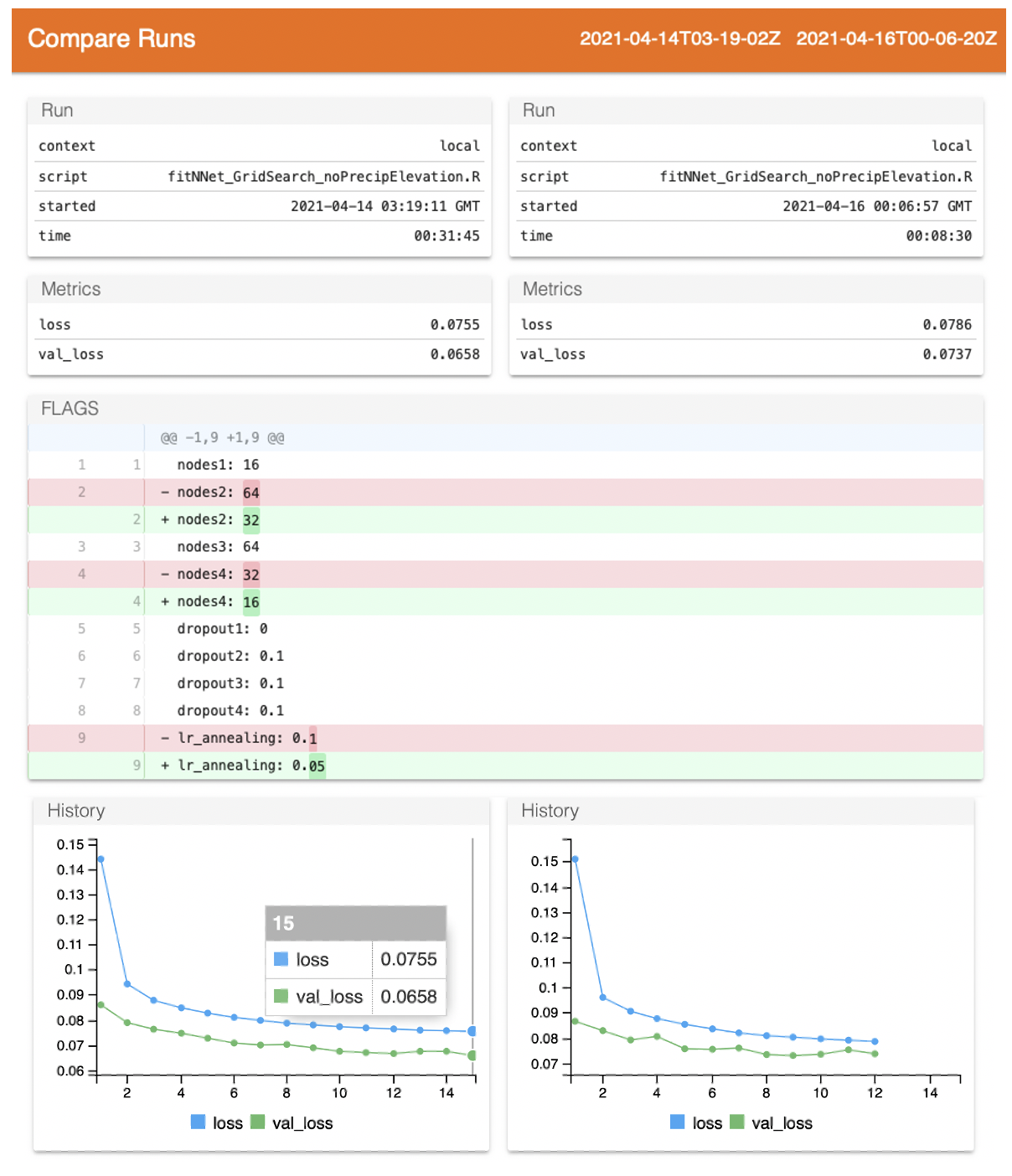
This launches a page similar to Tensorboard, providing basics about the runs and their loss metrics. The Github-esque track changes shows that nodes1_ has the same value between runs, but _nodes2_ has 64 for the first run and 32 for the second run.

The dropout rates are interestingly all the same between the two runs–and low–suggesting the model requires relatively little dropout. If all of the top models show low levels of dropout, I might fix them and instead shift focus to the learning rate or nodes tuning. There are also many more modeling options to consider, like the optimizer choice.

What else can we tell from the model runs? Below I plot the distribution of validation losses across the n=104 runs, each representing a different combination of hyperparameter values.

hist(ls_runs(order = metric_val_loss, decreasing = F, runs_dir = '.')$metric_val_loss, 
	breaks = 9, 
	las = 1, 
	xlab = 'Validation Loss', 
	main = 'Validation Loss Across\nDifferent Hyperparameter Combos', 
	col = 'plum2')

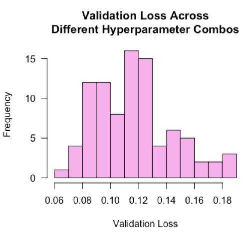
The losses are roughly normally distributed with a mean of 0.12. This tells us that a typical ‘blind’ guess at the hyperparameter values would land around a loss value of 0.12. Our best model’s loss is nearly half of that, suggesting the hyperparameter tuning improved model performance by 50%! I would be curious to see in practice if distributions are typically normal, and in the case when they aren’t normal, what that might tell us.

Tips

1. Run the model with default values first to get a sense of the expected computation costs.
2. Randomly sample hyperparameter value combinations rather than searching all possible combinations. When looking at the results, you may find that certain hyperparameters gravitate towards the same value. Fix those values, then perform a more exhaustive follow-up search on the remaining hyperparameters.
3. Similar to #2, the random search may tell you that, for instance, a value between 0 and 0.2 tends to be better for a dropout rate. Then you can narrow your search over just that span for follow-up searches. Repeating this process to narrow the windows for each hyperparameter is essentially a brute-force Bayesian search optimization.
4. By comparing the best and average performers from your search, you can see what the opportunity gap is for hyperparameter tuning. If it is negligible for your end goal, you can focus your efforts elsewhere.