RiverHeatNet: Building a river temperature neural network with Keras functional API

Motivation

I came upon the Keras functional API after setting out to develop a model for predicting river temperatures and their response to climate change. The dataset I collected consists of over 4.1 million temperature measurements across 1,210 rivers. Input variables like air temperature and precipitation are of the same time series structure as the output, but I also have information about each of the rivers like elevation and ecosystem type that I know are relevant and would like to incorporate.

The modeling challenge is that the predicted variable, water temperature, is a time series, while the input variables are a mixture of time series and static variables.

There are a few options for tackling this variable mismatch:

1. Use an ANN and ignore the time series aspect. Pros: Fast and easy. Cons: Lower accuracy since it leaves out so much useful information.
2. Use a recurrent neural network with the static variables converted to time series, repeating the same values at every time step. Pros: Incorporates time series information. Cons: Woefully computationally inefficient.
3. Combine the best aspects of #1 and #2.

Every neural network developed for river temperatures I have come across in the literature has gone with Option #1, sidestepping the modeling challenge by ignoring the time series structure of the data. This leaves a great opportunity to improve upon existing models. By the end of this post, you will see how I developed a model that flexibly incorporates both time series inputs and static inputs to predict a time series output using the Keras functional API.

Keras Functional API

Thanks to the Keras functional API, it is remarkably easy to combine recurrent neural network layers with standard, fully connected ANN layers.

The functional API can build all of the same models as the sequential API but has much greater flexibility to incorporate different inputs. The functional API can also be used to build models with multiple outputs such as combined classification and regression tasks (e.g. this image is a cat predicted to be 4.3 years old). I experimented with multiple outputs and the functional API when building a network for wildfires, combining a binary detection task (fire, no fire) and a regression task (if there is fire, what is its magnitude?).

Model Architecture

LSTM Layers

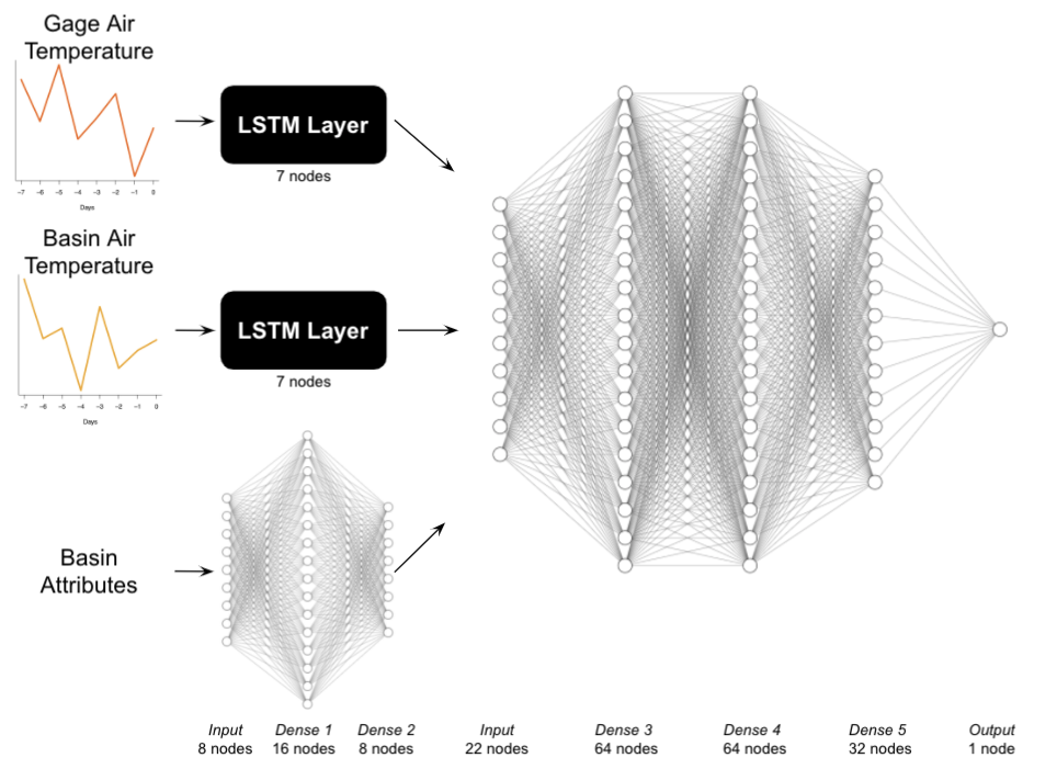
I feed all input variables that are time series (two distinct air temperature time series and a precipitation time series I later dropped) into separate long short-term memory (LSTM) cells. LSTMs, first proposed in 1997 by Sepp Hochreiter and Jurgen Schmidhuber, are a type of recurrent neural network commonly used in time series applications. LSTMS are capable of taking the input, storing it for as long as needed, and extracting its value later. As a result, they have been very successful in tasks with long-term patterns like speech recognition and long texts. A commonly used alternative is the gated recurrent unit (GRU), which can be easily swapped in the API.

airTLayer <- airTInput %>% 
  layer_lstm(units = 7, dropout = 0.15, recurrent_dropout = 0.15)

The code above gives an example LSTM layer for one of the input time series, the local air temperature. I likewise created separate layers for the basin-wide average air temperature and precipitation.

The units argument determines the dimensionality of the output space. I set it to 7 days. The input data are organized such that the ‘lookback’ period is 7 days as well, meaning that the model can only see data from the previous week when trying to fit today’s value. I chose the lookback period based on a literature review, where we have little reason to believe river temperatures from more than a week prior will give useful information about todays temperature. The output dimension of 7 days is a tuneable hyperparameter and does not need to match the lookback period.

The two dropout specifications impose a moderate regularization effect to help mitigate overfitting. How does it work? Simply put, during each forward or backward pass of the algorithm, 15% of the nodes are randomly ignored. This 15% level is also a tuneable hyperparameter, and for this dataset I found that 15% was actually too high.

Fully connected layers

For the 8 time-invariant basin attributes, such as elevation for a given sampling location, I fed them into a standard, fully connected ANN with two layers. Since I only have 8 basin attributes to feed in, the layers do not have many nodes.

## Basin attribute layer
nAttr = 8
siteAttrInput <- layer_input(shape = nAttr, name = 'siteAttr')
siteAttrLayer <- siteAttrInput %>%
  layer_dense(units = 16) %>%
  layer_activation_leaky_relu() %>% 
  layer_batch_normalization() %>%
  layer_dropout(rate = 0.1) %>% 
  
  layer_dense(units = 8) %>%
  layer_activation_leaky_relu() %>% 
  layer_batch_normalization() %>%
  layer_dropout(rate = 0.3) 

The code above sets up the basin attribute layer, feeding it into two layers. For each layer I use the leaky ReLU activation function, a typical default choice, along with batch normalization, which helps prevent overfitting and accelerate training. I also use dropout in each layer, with the dropout rates selected via grid search (more on that later).

Merge LSTM and fully connected layers

Next, I combine the different LSTM and basin attribute layers into an additional set of three fully connected layers. The output is the current day’s water temperature at a given river. Keras makes this very straightforward.

## Merge Input layers
concatenated <- layer_concatenate(list(airTLayer, airTlocalLayer, precipLayer, siteAttrLayer))

Just like that, the code above merges the different layers, which I then feed into follow-on fully connected layers:

## Define layers following concatenation
waterTOutput <- concatenated %>% 
  layer_dense(units = 64) %>% 
  layer_activation_leaky_relu() %>% 
  layer_batch_normalization() %>%
  layer_dropout(rate = 0.5) %>% 
  layer_dense(units = 64) %>%
  layer_activation_leaky_relu() %>% 
  layer_batch_normalization() %>%
  layer_dropout(rate = 0.5) %>% 
  layer_dense(units = 32) %>%
  layer_activation(activation = "linear") %>%
  layer_dense(units = 1) %>%
  layer_activation(activation = "linear") 

Why so few layers? Compared with the top networks designed for ImageNet classification, which can have hundreds of layers, this is indeed a simple and ‘shallow’ model. It is not for lack of data either, which would necessitate a simple model. Instead, I chose a handful of layers because the underlying task is relatively simple, controlled by physical relationships (hotter air = hotter water). The number of layers should correspond loosely with how complex you imagine the task is. Identifying faces, for instance, is far more complex a task than predicting temperature.

At this point we are pretty much done 💃 🕺!

## Compile model and add final specs
model <- keras_model(list(airTInput, airTlocalInput, precipInput, siteAttrInput), waterTOutput)

model %>% compile(
  optimizer = optimizer_adam(),
  loss = 'mse'
)

The code above compiles the model, telling it what to expect as inputs and outputs, along with specifying the type of optimizer for training and the loss metric (mean-squared error).

Hyperparameter tuning

Choice of hyperparameter values, such as dropout rates for each layer, type of optimizer, and numer of nodes can make a huge impact on model performance. Unfortunately, there are ‘rules of thumb’ for these at best, so it is often best to let the data tell you what to choose. I performed a grid search across potential values to make my final choices, aided by the tfruns package created by the TensorFlow community, which I’ll save for a different post.

Model evaluation

I set up an over-the-top set of steps for evaluating model performance, including three distinct test sets serving different purposes. But I won’t go into that here–it is all documented in an upcoming river heatwave manuscript. The quick version is that R² values were very good, on the order of 90% for test data consisting of rivers not used in training.

Final thoughts

I wrote this post in part because so many of the online tutorials I have seen use the Keras sequential API. However, in most of my work, I have eventually needed to add more customization and make the switch to the functional API, to the point where I now use the functional API as my default.

The code above is in all in R. I have used the Keras functional API in both R and Python, and the syntax is nearly identical. This makes deployment, migration between languages, and finding debugging solutions online a breeze.